REW's RT60 Decay graph provides a way to examine reverberation time behaviour at much higher frequency resolutions and with much narrower octave fractions than is usually possible, even at low frequencies, thanks to a frequency domain approach.

REW's RT60 Decay Graph takes a frequency domain approach to estimating RT60, rather than the more usual time domain approach.
Reverberation times are usually determined through time domain processing. The various RT60 values are estimated by calculating the slope of the Schroeder integral, which is a plot of the energy (squared values) of the impulse response that is backwards integrated (summed starting from the end and moving backwards). The different RT60 measures (e.g. T20, T30, REW's Topt) are then derived by calculating the best fit line to the Schroeder integral over different ranges. There are some limitations to this approach. The measurement's noise floor affects the shape of the Schroeder integral, causing it to curve. Various measures are applied to reduce that affect by estimating the level of the noise floor and altering where the integration starts and the initial values it uses. In addition, the octave band filters have group delays, which may affect the calculated reverberation times, particularly at low frequencies. The filters also usually have poor frequency discrimination, since their order is generally low (6th order typically) to avoid exacerbating the group delay problem. Strong resonances consequently have a masking effect on nearby regions of the response.
Reverberation times may also be estimated through frequency domain processing, examining the decays of the slices of a set of Short-Time Fourier Transform (STFT) plots. These are commonly used to produce waterfall or spectrogram graphs. The slices of an STFT series can be octave band filtered in the frequency domain using brick wall filters with no associated time domain group delays. Frequency discrimination is then determined by the characteristics of the window used for the STFT, the deciding factor generally being the width and shape of the left side of the window (aka the window rise time). Processing in the frequency domain makes it straightforward to present results using much narrower octave band filters, allowing individual resonances to be distinguished with no negative impact on the reverberation time estimate.
The Schroeder integral is not applicable to frequency domain processing. The STFT slices capture the reverberant decays and noise, reverberation times may be estimated by fitting an exponential decay plus noise function to the data series formed by the slice values at each time step. The fitting process must take into account the effect of the left window on the data series, where its width is more than the slice interval. It must also be tolerant of the non-monotonic nature of the decay data.
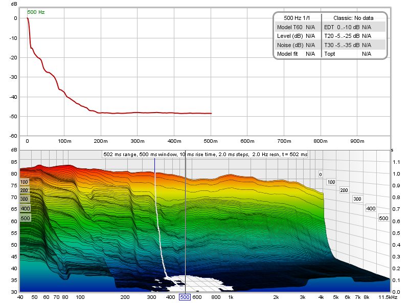
Here is an example of an RT60 decay plot after generating the STFT data (by pressing the Generate button in the bottom left corner of the lower graph) but before calculating the RT60 model. The upper panel shows the decay curve for the cursor position in the lower graph.
The control panel in the lower graph has a button to calculate the RT60 model.
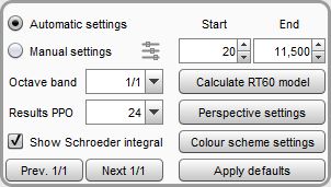
On the left side of the panel are controls for the STFT data. When Automatic is selected REW will determine the rise time, window width and time span to use for the STFT plot. Manual allows those settings to be altered, using the button to the right of the Manual selection. Octave band is the width of the octave band filter applied to the STFT data, while Results PPO determines the frequency resolution at which REW will calculate the model (up to 96 PPO). Show Schroeder integral allows the Schroeder integral for the nearest classical RT60 calculation result to be shown alongside the decay profile. The Prev. 1/1 and Next 1/1 buttons move the cursor to the previous or next 1 octave centre frequency.
On the right side of the panel are the frequency range over which the model fit will be calculated and the Calculate RT60 model button which runs the calculation. Perspective settings brings up a dialog to control the presentation of the STFT data while Colour scheme settings brings up a dialog to control the colour scheme.
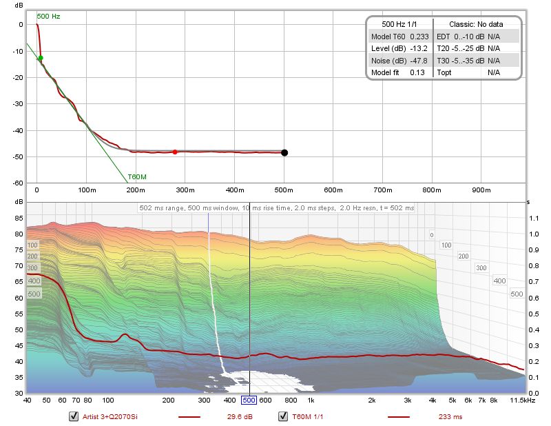
After the model has been calculated for each frequency the model result (T60M) will appear as an overlay on the STFT data, using a time axis on the right hand side of the plot. It can be shown or hidden by selecting or deselecting the T60M trace in the graph legend. In the upper graph the model result is shown as a grey curve, with a regression line corresponding to the calculated RT60 value shown in blue. The data panel shows the T60 time, the starting level of the model curve, the noise level and the model fit error (the lower the value the better the fit). Three dots are shown on the decay curve. Green and red indicate the start and end of the range used for the model fit. Black indicates the point past which REW considers the data not to be valid.

If classical RT60 results are generated for the measurement (from the RT60 graph) those figures will appear, along with the Schroeder integral and its regression line if they have been selected for display.
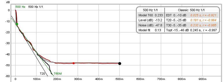
In this example the classical T20 RT60 value is lower than the model value. That is common in responses that have sharp early decays, as may be the case in heavily treated spaces. The -5 dB point on the Schroeder integral which is the starting point for T20 and T30 values is still within the early decay, so biases the results.
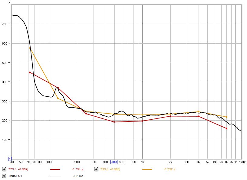
After the model has been calculated the result can also be viewed on the RT60 graph, allowing easy comparison with the classical measures.
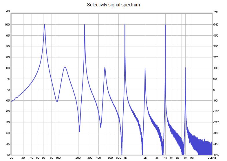
To aid in testing the selectivity of classical and frequency domain approaches a synthetic test signal was generated, consisting of equal amplitude exponentially decaying cosines at the one octave centre frequencies, with noise added at -60 dB relative to the cosine amplitudes. The cosine 60 dB decay rates alternate between 1.000 s and 0.100 s. Here is the spectrum of the test signal.
The signal will be octave band filtered in both approaches. We will first look at the classical approach, starting with the 6th order filters typically used.
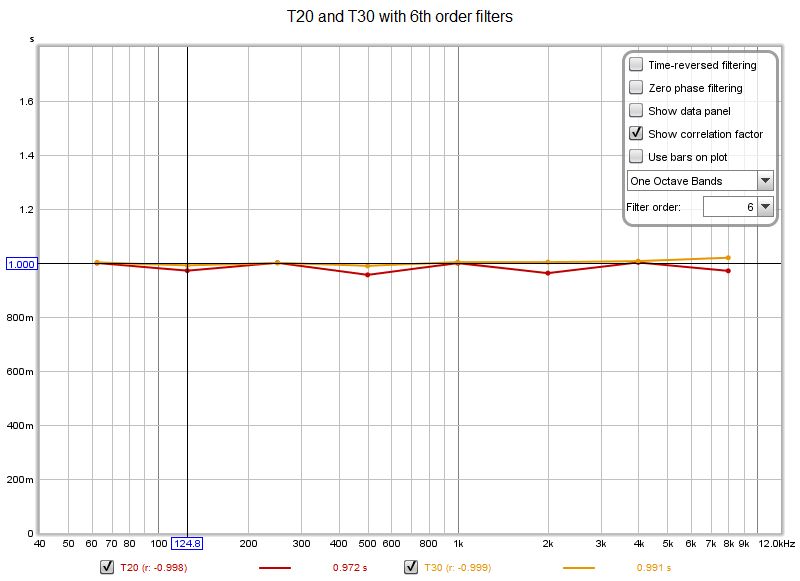
With 6th order filters the 0.100 s decays are not resolved at all. Next we will try 12th order filters.
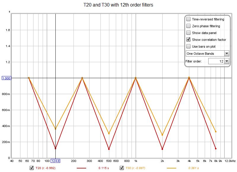
The 12th order filters are beginning to resolve the 0.100 s decays, but the results are still some way off. Next up is 18th order.
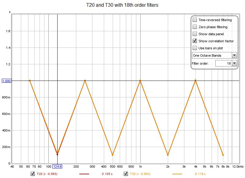
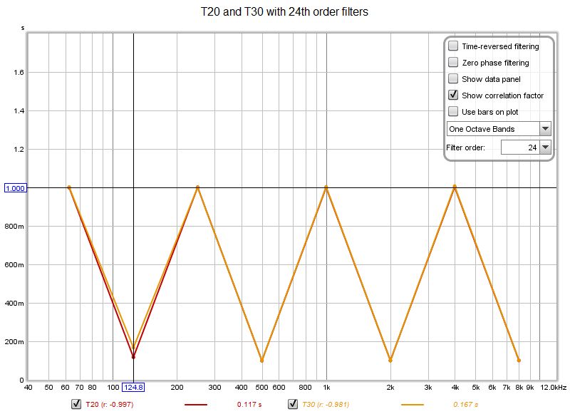
The 18th order filters have done the trick except for the lowest 125 Hz 0.100 s decay, with T30 still slightly worse than T20 there. Increasing filter order further makes the results worse rather than better, as the filter group delays begin to bias the results.
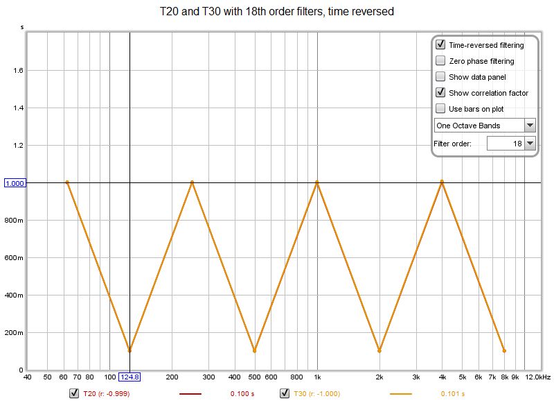
Perfect results can be obtained with 18th order filters and time reversed filtering.
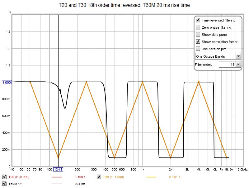
The frequency domain result depends on the window settings used. By default REW picks a 20 ms rise time for this signal, giving the following results (calculated at 96 PPO rather than only at the octave centres).
A 100 ms rise time improves the T60M performance, though it still can't quite match the classical approach with 18th order time reversed filters at the 125 Hz octave centre.
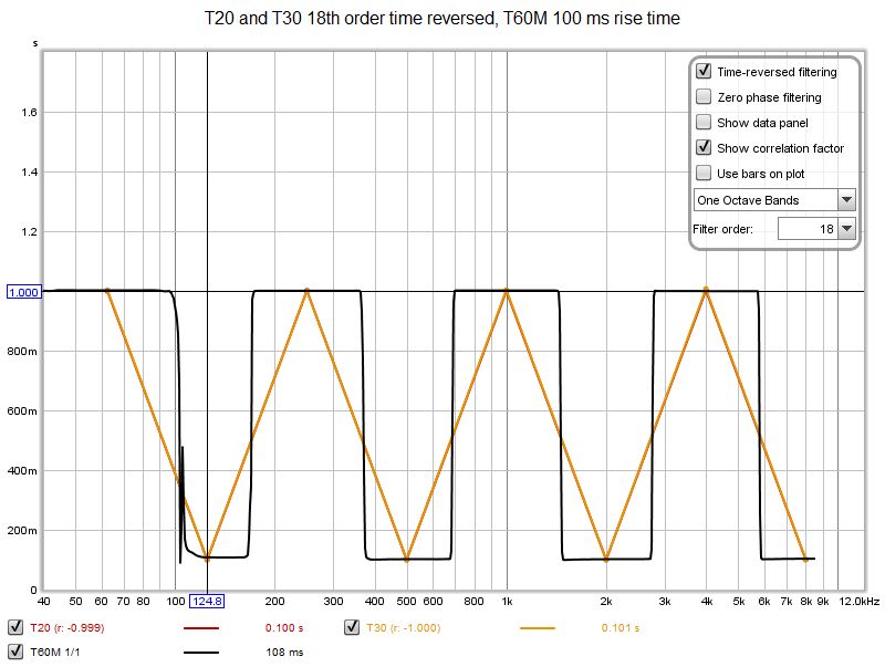
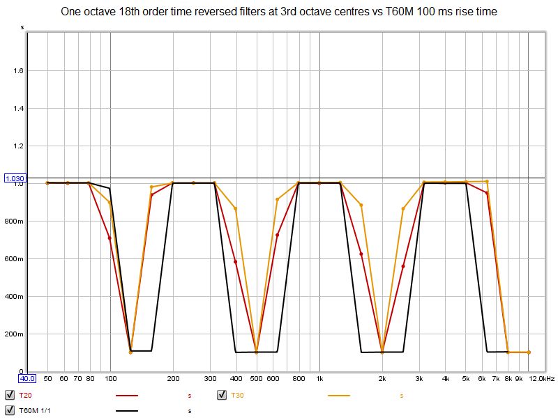
Further increases in T60M rise time improve the selectivity but degrade the accuracy of the RT60 calculation due to the effect using windows wider than the decay time has on the decay data. Nonetheless this is good performance from the alternative approach, particularly if we compare the behaviour of both approaches away from the one octave centres. The plot below uses 1 octave filter bandwidth, 18th order time reversed for T20 and T30, but also evaluates the result at the intervening one-third octave centre frequencies. T60M performs far better.
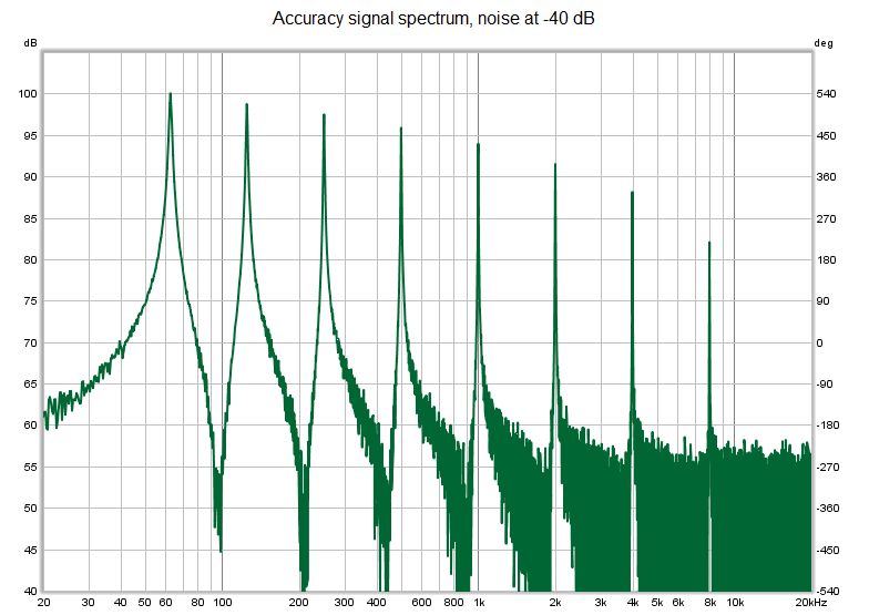
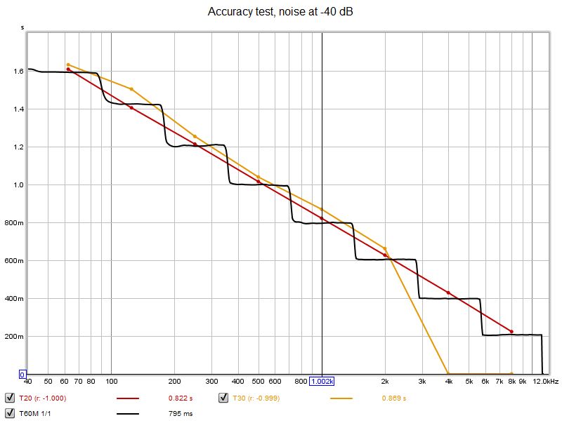
The next test is of accuracy. Another synthetic test signal was generated, again consisting of equal amplitude exponentially decaying cosines at the one octave centre frequencies, but with 60 dB decay times that varied in 0.2 s steps from 1.600 s at 63 Hz to 0.200 s at 8 kHz. Noise was added at two different levels, -80 dB to act as a clean signal reference and -40 dB to test performance in the presence of noise, in both cases relative to the cosine amplitudes. Here are the spectra of the test signals.
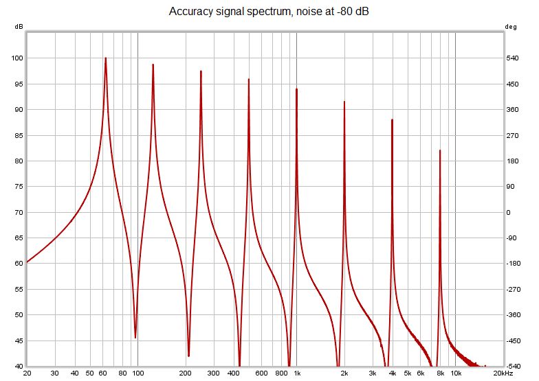
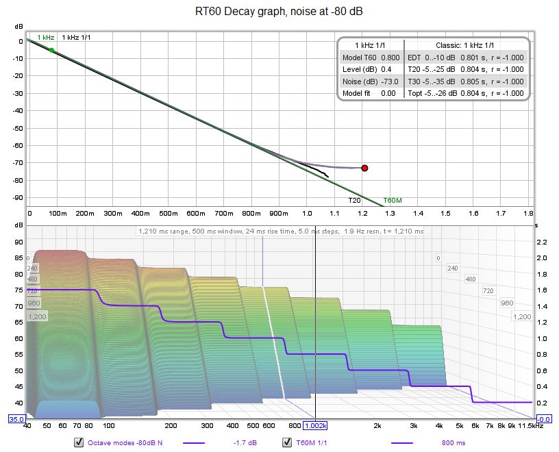
The signal with noise at -80 dB presented no difficulties for the new or the classical approaches.
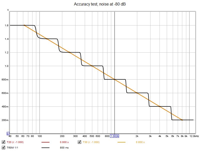
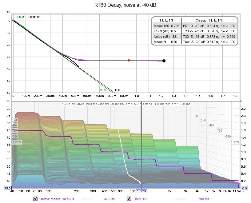
The signal with noise at -40 dB was more challenging for the classical approach, despite successful detection of the noise floor (using Lundeby's method) in all cases. Filter order made negligible difference, 18th order providing a very slight improvement. The results below are for 18th order filters. The T60M frequency domain approach performed significantly better than the classical approach with this signal.
Here are examples of the RT60 Decay graphs for both cases.
Here are some technical details of REW's implementation of the RT60 Decay analysis.
The decay data is derived from a series of Fourier Transforms, referred to as slices. The first slice uses the peak of the impulse response as the reference point, each subsequent slice is shifted in time by the slice interval. The total time span covered by the slices is the "Range" setting. Each slice is windowed with a left side Hann window of width equal to the rise time and a right side Hann window equal to the "Window" width. Note that at high frequencies the noise floor of the frequency domain approach is typically higher than the classical approach, due to the FFT window width required for the low frequency range. Narrower windows and shorter rise times could be used to generate high frequency decay data with lower noise floors. A frequency-dependent windowing (FDW) approach could be considered, but FDW implementations typically have symmetric windows which would result in excessive rise time at low frequencies.
The Automatic settings derive the time range by carrying out a conventional T20 analysis using 1 octave 6th order filters at 250, 500 and 1000 Hz. The longest T20 figure is used as the time range, with a minimum range of 500 ms. The slice interval is set to provide about 250 slices over the range, with a maximum slice step of 100 ms. The rise time is set to 2% of the range, with a maximum of 400 ms.
The data for each slice is low pass filtered to 1/48th octave then sampled at 96 points per octave to provide a log spaced data set. Subsequent octave band filtering is applied to the squared magnitudes of that log spaced data, using a kernel that is unity across the band width except at each end, where the kernel amplitude is 0.5.
The data series formed by the values of each slice at a frequency is analysed for the RT60 calculation. An initial scan of the data is carried out to determine if there are sharp roll offs or rises near the end of the data, if found subsequent data are excluded from the analysis.
The analysis consists of fitting a decaying exponential plus noise function to the data. The function is:
f(t) = level*exp(-6*log(10)*t/t60) + noise
The three model parameters level, t60 and noise are determined by minimising an error function formed by the difference between the function value and the decay data at the slice times. REW uses the mean squared value of the difference between the dB decay data and the dB values of the model function, weighted by an error scaling function that gives less weight to values that are below -20 dB. Initial estimates for the model parameters are based on a least squares line fit to the decay data over the range from -10 to -20 dB.
The model error is evaluated over a sub-section of the decay data. The nominal start point for the model fit is the -5 dB point on the decay curve, but at least 10 ms or the rise time after the decay start, and with an overall limit of not being more than 10 dB down the decay curve. It should be borne in mind that, unlike a Schroeder integral, the decay data is typically not monotonic, so "-5 dB point" refers to the last point in the response where it passes through -5 dB. REW's adaptation of Lundeby's method is applied to the decay squared magnitude data to estimate the noise floor and the intersection of the noise floor and the RT60 decay line, the fit end index is then set twice as far into the decay curve as that intersection point. If the lundeby routine doesn't find a good result the fit end is the end of the valid data.
A Java port of UNCMIN (by Steve Verrill) is used to find the optimal model parameters. UNCMIN is an unconstrained optimiser, constraints are imposed by modifying the minimiser vector entries before they are used in the model function. That constraint process is part of a transformation of parameter values from the optimiser space to the function space. The parameters in the minimiser space corresponding to level and noise are scaled dB equivalents of the model values. The minimiser parameter corresponding to t60 is a scaled reciprocal of the T60 value. Limits are placed on the values based on the initial estimates.
Good selectivity at low frequencies requires rise times that are typically larger than the slice interval. The effect of the left window on the decay data must be taken into account before the model fit error is evaluated. The left window is convolved with the decay data, but not with the decay values at each slice themselves but rather with the differences between the decay values for successive slices, since it is that difference in the decay the window is acting upon.